GEOLOGY & GEOPHYSICS: Three-dimensional seismic object detection cutting cycle time

Fault example from offshore Africa. Time-slice from the fault cube.

Interpretation of 3D seismic data is a time-consuming task requiring advanced interpretation workstations and trained, exp-erienced personnel. In the last decade, numerous advanced tools have been deve-loped to assist the interpreter, who has to cope with ever-increasing data volumes. Improved visual-ization methods, such as 3D stereo vision and immersive techniques as well as seismic attributes and image processing techniques, have emerged as important tools to produce more accurate interpretations in less time.

The number of seismic attributes available on standard interpretation systems is constantly growing. Although this is considered a positive development in itself, we do identify problems with the interpretation of the ever-growing quantity of attributes:

• Only a few experts know what the attributes mean in geological/geophysical terms.
• Many attributes are not unique (different geological features have similar attribute responses).

Therefore, it is not sufficient to only look at one attribute. Instead, one has to use many attributes simultaneously. The obvious questions that arise are which attributes to use and how to combine them. Today, many interpreters display and compare multiple attribute cubes, while others try to combine these using some kind of mathematical expression.

In the first case, the interpreter must have a workstation capable of handling multiple volumes of attribute data and displaying them simultaneously. In the latter case, the interpreter must find a mathematical expression to combine the attributes effectively. Since seismic surveys of different vintages usually exhibit different characteristics, a mathematical expression between various attributes will only be valid for the vintage for which it was developed.

Instead of having a static mathematical expression between attributes, we use artificial neural networks to find relationships between the attributes and desired objects in the seismic data.

Methodology

Seismic section with a salt pillow.

Artificial neural networks are computing techniques that aim to emulate some desired properties of the human brain. One of these properties is learning from experience. Given a number of examples, an artificial neural network can be trained to learn the relationship between the inputs (a set of attributes and the desired output; is this a fault or not?).

The usage of the artificial neural network based object detection is straightforward and intuitive. The interpreter focuses on one geological object at the time. This can be seismic chimneys, faults, reflectors, stratigraphic features, hydrocarbon anomalies, and so on, basically any object that is relevant for seismic interpretation.

The first objective of our method is to enhance the contrast between objects and their background. The output is an "object probability" cube. With the help of modern visualization techniques, it is then possible to study the spatial relationship between different objects enhanced in this way. A second objective, which is beyond the scope of the current paper, is to extract objects (3D bodies and planes) from the enhanced cubes to facilitate geological model building.

Attribute volumes

The workflow for the generation of "object probability" cubes is as follows:

1. The interpreter scans the seismic data for the object of his/her choice. Let us assume that the objective is to map faults. Clicking on seismic sections and time-slices at recognized fault and non-fault positions then creates the required training set for the neural network.
2. Attributes with the potential to increase the contrast between object and background are selected. The selection process is based on common sense and visual inspection supported by statistical measurements such as correlation matrices and color-coding of neural network weighting functions. The latter is a simple and effective technique that assigns a color from a given color bar to the input nodes of the neural network. Higher weights mean that the network relies more heavily on the input node to predict the target value. The important attributes are thus easily identifiable. Default attribute sets exist for a range of geological objects to facilitate non-expert users.
3. The artificial neural network is trained to give an output of one at object locations and zero at non-object locations. The performance of the classification is measured by dividing the locations into two groups, one for training and one for testing the neural network. The quality of the result is expressed in a classification matrix.
4. The trained network is applied to all sample locations in the seismic data. The network gives an output value ranging between approx. zero and one. The output can thus be considered to represent the probability of the object of interest to be present at each location.

The technique described has been applied successfully to detect such object-types as gas chimneys, faults, and salt-bodies.

Gas chimneys and salt

Salt probability from the seismic section.

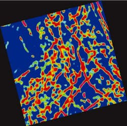
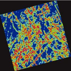
The first example is from a prospect evaluation study. The data are from the deepwater slope of Green Canyon in the Gulf of Mexico at about 2,000 meters water depth. The 3D seismic cube covers an area of approximately 5 km by 10 km. Seismic chimneys, a salt dome, amplitude anomalies, and mapped horizons are the objects of interest. Horizons were mapped using conventional techniques. The amplitude anomalies are shown as single attributes.

These objects have similar characteristics and therefore cannot be separated effectively by single attributes. For example, chimneys and salt are both characterized by low energy, low trace-to-trace similarity (or coherency) and a chaotic behavior of the seismic response. The latter feature is captured by an attribute we call "dip variance." In a small cube around the extraction point, the statistical variance of the local dips and azimuths are calculated to derive the "dip variance."

To distinguish salt from chimneys, we use the so-called "directivity principle" when we create attribute sets for chimneys and salt. Geometrical aspects of the bodies, such as size, shape, and notably directions, are used to increase the contrasting power of the attributes. Attribute sets are made directive by specifying attribute windows and by using multiple windows aligned in the direction of the object.

With chimneys, this is simply done by extracting the same attributes in three vertically aligned windows around the evaluation point. The network can thus learn that we are looking for a vertical disturbance of the seismic response.

For salt, we use only one extraction window, but we also give the in-line, cross-line and two-way-time location of the evaluation position, to reflect the fact that salt does not occur anywhere in 3D space, but is confined to a particular corner around the example locations.

Unraveling US Gulf

Massive oil and gas seepage is taking place over the entire northern slope of the Gulf of Mexico. This is evident from geological, biological, and satellite data. The most pervasive seepage seems to occur in the deepwater slope areas, rather than on the shelf (Jean K. Whelan, Sea Technology, September, 1997). Seafloor features that have been associated with hydrocarbon seepage in the Gulf of Mexico include carbonate mounds, mud volcanoes, and seabed depressions. Seismic chimneys are commonly correlated with hydrocarbon seeps.

By enhancing seismic chimneys through the method described above, it becomes feasible to interpret hydrocarbon migration paths and unravel the hydrocarbon system. Detailed studies help to identify where hydrocarbons originate in the geological sequence, how these hydrocarbons migrate upwards, become trapped, and spill out to reach the surface. Chimney interpretation is therefore a useful tool in the exploration phase, but it also can provide valuable information at later phases of a field's life cycle (regarding fault sealing and compartmentalization).

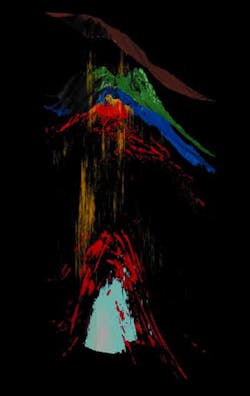
The three mapped surfaces in an accompanying figure are displayed as time maps in blue, green, and brown. The upper one represents the seabed. The second one is mapped at about 200 meters sub-seabed, and the third at 400 meters sub-seabed. From the standard seismic cube, only the highest amplitudes are displayed in red. Lower amplitudes are made transparent in this display. Chimneys from the chimney cube are displayed in yellow. These correspond to the high values in the cube (high chimney probability). Lower values are made transparent. The salt is displayed in bluish-white. The shallow cloud of high amplitudes (red) is interpreted to represent a hydrocarbon charged reservoir.

Chimneys surrounding the salt dome are interpreted to indicate upward fluid migration from a deeper reservoir. The high density of shallower chimneys indicates charging of the shallow reservoir. The sub-seabed surfaces (green and blue) exhibit a radial fault pattern caused by the upward movement of the salt dome.

Chimneys are visible up to the seabed. A small mound is present at the seabed close to the top of the shallowest chimney on the left-hand side. This may be a small mud volcano generated by transport of sediments, fluid, and/or gas to the seabed.

Faults and salt

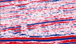
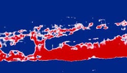
Mapping faults is usually one of the most difficult and time-consuming tasks in seismic interpretation. In a typical work flow, the initial goal is to establish a structural framework by mapping the larger faults first. Detailed mapping of smaller scale faults at the reservoir interval follows this. The example shown is from an area offshore Africa.

The same method used to enhance chimneys was used here to detect faults. Similar attributes were used, but attribute parameters and window settings were tuned to faults rather than chimneys. The multi-attribute, neural network-based approach shows better fault continuity and a higher signal/noise ratio.

Mapping the exact outline of a salt dome is important for structural mapping and accurate time-depth conversion. In pre-stack depth migration exercises, a geological model must be updated repeatedly, and it pays to incorporate a fast and accurate mapping procedure. The example from onshore Western Europe shows a Zechstein salt pillow. The boundary between salt and overlying/underlying formations is quite sharp.

Salt has moved upward and has possibly squeezed into the overlying strata at various positions along the top of the salt small domes. These proto-salt domes seem to coincide with weaker zones in the overburden where faults are observed.

The method of seismic object detection has proved to reduce interpretation times drastically, and numerous geological objects such as salt, gas-chimneys, and faults can be interpreted more rapidly and more precisely than with manual methods. In the first example, the presence and distribution of chimneys in the area make the presence of a deep and a shallow hydrocarbon charged reservoir more likely. A manual mapping of chimneys would have been difficult, less precise, and more time consuming. The second example shows that faults can be mapped more accurately by the method than by conventional, single attribute techniques. The last example shows that salt bodies can be delineated in great detail.

Acknowledgement

Bert Bril of dGB and Paul Meldahl of Statoil are co-inventors of the seismic object detection method.