Offline wells reduce value in US deepwater Gulf
Nimi Henderson
Thomas Shattuck
Wood Mackenzie
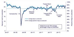
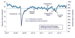
Wood Mackenzie recently studied the number of days of production per month for more than 1,200 wells indeepwater Gulf of Mexico (GoM) between 2007 and 2013. Production wells are thought of as flowing more or less consistently. However, these wells can be shut-in for numerous reasons, including inclement weather, equipment failure, and on-going maintenance drilling programs like workovers, side tracks, and recompletions.
Based on the study, producing oil and gas wells in deepwater GoM were online on average only 79% of the time – less than 10 months in any given year. While it is intuitive that a loss of production leads to lower revenue in the near-term, there is also a long-term impact as oil and gas production is deferred. Reducing uptime decreases oil and gas fields' net present value (NPV) and internal rate of return (IRR). For a larger field in deepwater GoM, less than a 10% change in producing days each year leads to as much as a 15% change in NPV. For Wood Mackenzie's base case model Lower Tertiary field with a valuation of $822 million, this is the equivalent of $100 million in unrealized returns.
So while the average well in the region has been producing the equivalent of 24 days per month, there is substantial underlying variation from well to well and year to year. The standard deviation was approximately 10%, or roughly three days. However, there are occasional periods when the majority of wells are not producing simultaneously. For example, after Hurricane Ike a majority of the fields were shut-in for months due to damage to production facilities and infrastructure. During this time, the average number of days per month on production dropped below 20% in September 2008 and did not exceed 60% until January of the following year. Hurricane Katrina had a similar effect on production three years earlier.
Despite there being only one major hurricane between 2007 and 2013, Ike was severe enough to shut-in the majority of deepwater wells for almost four months. If Ike is excluded, the six-year average increases from 79% to 81%. This does not reflect the variation in shut-in duration from well to well. Operators with sufficient contingency plans for pipeline and facility damage as well as logistical limitations can bring their wells online faster than the average. For example, oil exported via Shell's Auger pipeline system was re-routed through a temporarily reversed section of the Poseidon pipeline following Ike. Fields without that flexibility could be shut-in for infrastructure repairs after future hurricanes.
While weather related shut-ins are inevitable, there are other times where wells or entire fields go offline. Whether due to maintenance, workovers or equipment failure, these also impact the field's economics. Subsea tiebacks have an increased risk of being shut-in because of problems or maintenance at the host facility. Although these shut-ins are also unavoidable to some degree, operators can design maintenance and workover programs to minimize downtime and to increase a producing asset's value.
Eliminating downtime
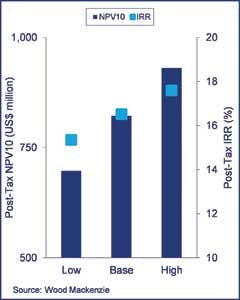
To illustrate how changes in days of production per month affect the value of different types of fields in GoM, compare two model fields under varied risking conditions. One is a multi-well, Lower Tertiary field, similar to BP's Kaskida (KC 292) or Chevron's Jack (WR 759). The other is a single-well, Middle Miocene subsea tieback, similar to those in Noble Energy's Rio Grande complex.
The Lower Tertiary model assumes a standalone facility with 12 producing wells and three water injectors with recoverable reserves of 300 MMboe. The Middle Miocene model assumes a single-well tied back to a nearby facility with total recoverable reserves of 22 MMboe. The base case assumes 10 months of production per year during the entire life of the field, whereas the low and high cases assume nine and 11 months, respectively. Assume the same recoverable reserves for the low, base, and high cases.
Asoil and gas production is deferred into the future, the NPV and IRR for each field is reduced in real terms. For a base case model Lower Tertiary field, the NPV is $822 million and IRR is 16.5%. An additional month of production each year increases the NPV by $100 million and IRR by 1%. These effects also increase with field size. In the case of the largest Lower Tertiary field modeled, Tiber at 566 MMboe, producing for 11 months a year increases the valuation by over $300 million.
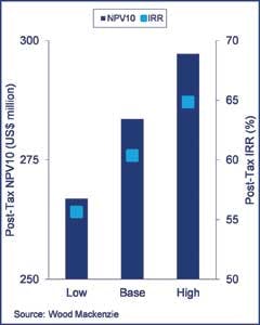
For a model Middle Miocene, single-well subsea tieback, the base case NPV is $284 million and IRR is 60.4%. An additional month of production each year increases the project valuation by $15 million and increases IRR over 3%. For a multi-well tieback, the change is proportional. A three-well tieback can see an increase NPV more than $50 million.
In the low case, production in earlier years is reduced and field life is extended, decreasing near-term revenue and increasing total operating costs. For the model Lower Tertiary field, producing the equivalent of nine months a year reduces NPV by 15% or $125 million. For the Middle Miocene field, NPV drops by 6% or $17 million. In both cases, the downside of losing a month of production a year outweighs the increased value from producing an extra month. To mitigate these risks, operators may choose to shorten field life and recover less reserves. However, this still likely reduces the overall valuation of the field.
Although three days a month seems like a small number, over the period of a larger field's life, this can defer production by years. In cases like Hurricane Ike, shutting-in production is unavoidable, but the effects can be mitigated by developing adequate contingency plans to bring production on sooner. Beyond that, optimizing maintenance, workovers and side tracks to limit non-productive time can improve a field's economics and increase earlier cash flows. Furthermore, operators should review redundancy and reliability of production equipment to limit time-consuming maintenance and preserve value in the long term.
Modeling assumptions: The models used for the generic Lower Tertiary and Middle Miocene fields evaluate a development project sanction forward.
The Lower Tertiary model assumes sanction in 2018 with first production in 2023 and the field developed via a standalone, wet-tree facility with third-party built oil and gas export lines transporting hydrocarbons to shore. The field was assigned recoverable reserves of 300 MMboe.
The Middle Miocene model assumes sanction in 2016 with first oil in 2018 and the field developed as a single-well subsea tieback to nearby infrastructure. The field was assumed to have recoverable reserves of 22 MMboe.
The low, base, and high cases were generated by varying the number of months a year a field was producing, from nine to 11 months. The field life varied between cases; however, all wells were permanently shut-in after oil production dropped below 300 b/d.
Economic assumptions: Wood Mackenzie's discount rate is 10% nominal. The discount date is Jan. 1, 2014, and the inflation rate is 1.9% in 2014 and 2% from 2015 onward.
Wood Mackenzie's Brent oil price assumption (nominal terms) is $103.25/bbl in 2014, $100/bbl in 2015, $98.73/bbl in 2016, $98/bbl in 2017, and $97.42/bbl in 2018, inflated at 2% per annum thereafter. This equates to a long-term Brent price assumption of $90.00/bbl (real, 2014 terms) from 2018 onward.
Crude from the model Middle Miocene field is assumed to trade at parity with LLS crude at (nominal terms): $98.73/bbl in 2014, $96.38/bbl in 2015, $95.29/bbl in 2016, $94.30/bbl in 2017, $93.72/bbl in 2018, inflated at 2.00% per annum thereafter.
Crude from the model Lower Tertiary field is assumed to trade at parity with Mars crude at (nominal terms): $97.75/bbl in 2014, $95.86/bbl in 2015, $95.42/bbl in 2016, $95.67/bbl in 2017, $90.94/bbl in 2018, inflated at 2% per annum thereafter.
Wood Mackenzie's Henry Hub gas price assumption (nominal terms) is $4.31/Mcf in 2014, $4.20/Mcf in 2015, $4.72/Mcf in 2016, $4.73/Mcf in 2017, and $4.74/Mcf in 2018, inflated at 2% per annum thereafter. This equates to a long-term Henry Hub price assumption of $4.38/Mcf (real, 2014 terms) from 2018 onward.