Online tool enables quick evaluation of tieback options
Elka Lacno
John D. Grace
Earth Science Associates
The importance of subsea tiebacks in the deepwater Gulf of Mexico emerged and continues to grow motivated by three quite immutable trends. First, the average size of new discoveries has fallen, reducing the economies of scale afforded by the early, very largest fields. Therefore, fewer new fields can support stand-alone platforms.
Second, new discoveries are in increasingly deepwater. Despite cost-saving improvements in technology, deeper water almost always means higher development, production and transport costs.
Finally, a growing number of major deepwater platforms set over the last 20 years have, or will have, rising excess capacity as the production of their principal fields declines – it is cheaper to rent capacity than to build it.
As a result, evaluating a new project, even before bidding, increasingly requires examining tieback options. Here, we explain a tool and methodology for that analysis. Its workflow follows two stages: First, evaluate candidate destination platforms by estimated spare capacity. Second, determine a tieback path that minimizes cost through a trade-off between distance and slope, while recognizing and avoiding seafloor obstacles. The tool is executed through a web browser by GOM3, a specialized set of integrated data and tools built on a geographic information system (GIS) platform.
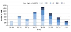
Number of deepwater (> 656 ft) wells in the Gulf of Mexico drilled by year and water depth between 1980 and the first half of 2017.
Route selection
If a company’s new prospect is close enough to its own platform, given sufficient capacity, where to send the anticipated production is simple. Much more often, a number of alternative destinations need analysis to develop a list of good choices. Ultimately, in-depth engineering and commercial study will be required, but listing candidate platforms’ estimated available capacities is the first step.
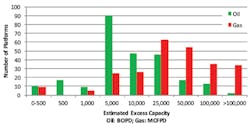
We estimate a facility’s current excess capacity by subtracting its highest monthly production in the preceding 12 months from its historical maximum. Oil and gas are calculated separately. This does not account for post-peak reduction of capacity or commitments by an operator to take production from other tieback projects but serves reconnaissance purposes. We also note whether or not the facility is currently producing as some platforms are still officially “active” and have high apparent idle capacity but may be in the process of demobilization.
Distribution of estimated excess capacity for oil (in barrels of oil per day, BOPD) and gas (in thousands of cubic feet per day) on platforms in greater than 656 ft water depth in the Gulf of Mexico as of Nov. 15, 2017.
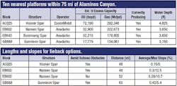
To illustrate the methodology, take as an example examining four tieback scenarios from a single hypothetical origin at 26.906°N and -94.218°W. This point is in 4,492 ft of water in block Alaminos Canyon (AC) 079, covered by lease currently held by BHP. On entering the origin location, the user is presented with a list of up to 10 of the nearest platforms within a maximum of 75 mi. They are sorted by distance and show the block, water depth, operator, estimated current excess capacities of oil and gas and current operating status. The operator is included because that data may inform the choice of destinations. In this example, three were chosen: from AC079 to the Hoover spar, to the Gunnison spar and to the Nansen spar.
Optimal route
Of course, the shortest path between two points on a plane is a straight line. However, the seafloor of the continental slope in the Gulf of Mexico is far from being a plane. Some areas cannot be legally traversed and others only at very high costs. Therefore, in searching for the shortest route, the user must immediately consider at least two additional factors: seafloor slope and obstacles.
The method for finding an optimal route is to form a mathematical network approximating the seafloor, its slopes and obstacles. The network is composed of nodes 328 ft apart on a square grid, each connected by eight edges representing potential pipeline route segments. Four edges connect to neighboring nodes to the north, south, east and west, which are 328 ft long and the other four edges are 464 ft long, leading to the four diagonal neighbors.
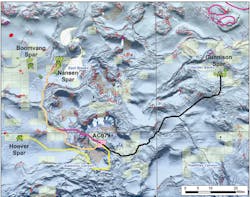
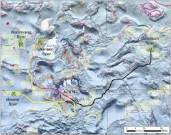
Four calculated tieback routes with a common origin in Alaminos Canyon (AC) 079 in 4,492 feet of water, currently leased by BHP (pink). There are two routes to the Nansen Spar: one avoids seafloor obstacles (magenta) and the other does not (light orange). The third route is to the Hoover spar (yellow) and the fourth is to the Gunnison spar (black). Light solid lines are existing oil (green) and gas (red) pipelines and umbilicals (yellow). The small irregular features of several colors are the boundaries of several classes of seafloor obstacles and the larger polygons are oil (green), oil/gas (green with red stripes) and gas (red) fields. Current leases are shown in semitransparent yellow.
A change in slope between two points on a pipeline route affects both the cost of pipeline construction and the energy required to move the liquids and gasses transported. Therefore, there is a tradeoff along any route between the length of the pipe and the slopes it must travel. The influence of slope is included in the model in two ways. First, based on a bathymetric grid in GOM3, each edge carries the seafloor slope between neighboring nodes as an attribute.
Second, using a slider in the interface, the user may input a “slope importance factor” (β,1≤β≤99) to weight the relative importance of slope versus distance in calculating the optimal path. Where the absolute value of the slope along an edge (measured in percent) is Ɵ and the length of the edge is d. This equation calculates the weight (w) assigned to each edge in the network.
Through the data in GOM3, seafloor obstacles are introduced into the network. They fall into three classes: regulatory no-go areas (e.g., marine sanctuaries), quarter-mile buffers around existing platforms and subsea structures and all known seafloor characteristics that may constitute hazards (e.g., mud volcanos, hydrates, active seeps). Computationally, edges that transect obstacle polygons are dropped from the network so they cannot be included in a candidate tieback route.
Given the node spacing, the network for the deepwater, US portion of the Gulf of Mexico contains 180 million nodes. For computational efficiency in calculating each route, the network is reduced to a subset along the straight-line path between the origin and destination. Generally, it is formed by first creating a rectangle with the origin and destination points at diametric corners. Then a 10-mile buffer is computed around the rectangle and all nodes outside the buffer are excluded. For example, by subsetting this way, the time to calculate a 50-mi tieback drops by a factor of 100.
Within the subset-network, starting at the origin node, an algorithm developed by Dijkstra (1959) is applied. This evaluates the eight edges surrounding a node, picking the lowest-weight edge and making the node connected to it the next evaluation point. That simple rule is then applied at the second node to find a third. At the third node, the algorithm then looks back and examines if there were any lower-cost paths to get from the first to third nodes (i.e., other than via the second). If not, the initial route from the first to the third is retained; if a cheaper (i.e., lower-weight) path exists, it is substituted. Given the least-cost way to get from the first node to the third, the process is then repeated until the optimal path from origin to destination is found. This method was implemented in Python.
As edge length and slope and the presence and areas of obstacles are all considered, the final path is optimal subject to these variables.
Smoothing the route
Given the grid arrangement of network nodes, the final path, even though mathematically optimal, is almost always very “jagged,” composed of short, straight segments. To create a more practical path, the optimal path from the process above is subject to a centered five-point moving average:
Eachxi,ȳi pair are projected coordinates of nodes along the smoothed path and N is the total number of nodes along the original pipeline path, composed of points xi and yi. This results in a smoothed path version of the optimal line between the origin and destination.
Output
Once the inputs are submitted, the algorithm generally takes several minutes to compute the solution and prepare a zip file emailed to the user. The file includes a report showing inputs, a map and the characteristics (e.g., length, average and maximum slope) of the optimal path. A .csv file is included with the path coordinates, which can be imported into Excel, CAD or other packages. So is a shapefile representing the optimal path; it can be added for further analysis with the other data and tools it contains or loaded into other packages that read shapefiles.
In the example above examining tieback routes from AC079 to the Hoover, Nansen and Gunnison spars, four cases were tested. Three used the default slope importance factor and were set to avoid seafloor anomalies. The fourth test was a second route to Nansen in which no provision was made for avoiding seafloor anomalies.
The alternative test of a no-obstacle-avoidance path to Nansen produced an apparently paradoxical result: the route avoiding obstacles is shorter than the one that does not. The reason is that the route avoiding obstacles was forced to take a higher-maximum slope route, 12.5%, to minimize length; the unconstrained route is longer but encounters a maximum slope of 10.7%. This type of influence in the trade-offs between slope, obstacle-avoidance and length can be explored further by changing the value of the slope importance factor and rerunning the analysis.
Future development
Going forward, we anticipate further development of the tie-back tool to include the following types of improvements, described below:
Cost. A rough cost could be estimated, either using available public data or user inputs. Costs could be refined by disaggregating seafloor obstacles and grading them from strict no-go zones to zones that can be transited but at a higher cost. Additionally, whereas only the absolute value of slope is currently used, positive and negative slopes could be weighted separately.
Excess capacity. The estimates of each platform’s current excess capacity could be expanded to include decline curve-based forecasts of future production from existing wells and thereby estimate future excess capacities.
Slope importance. Empirical estimates of the slope importance factor, statistically inferred from the paths of existing pipes, could be offered to the user as guidance.
Computation speed. To increase model speed, we are exploring further optimization of our network analysis algorithms and use of special-purpose hardware for the matrix manipulation the approach requires.
Conclusions
A web-based tool for reconnaissance evaluation of tie-back options from a prospect or discovery provides a first careful look at transportation options for new oil and gas volumes. Estimated excess capacity of proximate platforms not only filters unrealistic destinations but sets a foundation for expected tariffs from different platform operators. Likewise, the sensitivity of routing to seafloor characteristics, like slope and the presence of obstacles, affords quick evaluation of engineering options. Running the tool over the web brings it in line with the accelerating move to light, mobile software applications that used anywhere and can be easily updated.
References
Dijkstra, E.W., 1959, A Note on Two Problems in Connexion with Graphs, Numerische Mathematik, vol.1, no.1, pp. 269-271.
Acknowledgement
The authors wish to thank the other members of the project team at Earth Science Associates: Tony Dupont, Scott Morris and Deepal Saraf; and acknowledge the helpful discussions with Walter Stromquist.
The authors
Elka Lacno received her bachelor of science in mathematics and masters of science in applied statistics from California State University Long Beach. She joined Earth Science Associates as a Data Scientist specializing in network analysis, bidding theory and modeling auctions.
John D. Grace received his Ph.D. in economics for Louisiana State University and taught geology and mathematics at LSU, University of Southern California and California State University Fullerton. He began his career as a mathematical geologist at ARCO’s research lab then went to their corporate planning group. He has been president of Earth Science Associates since 1991 and is a member of the Society of Petroleum Engineers and Society of Exploration Geophysicists.
