Comparing towed, seabed 4D methods for Foinaven reservoir monitoring
Seismic reservoir monitoring over deep-water fields has the potential to deliver important information for managing the reservoir. When Foinaven, located 190 km west of Shetlands, was developed, the asset partners (BP and Shell) made an early investment in 4D (time-lapse 3D) seismic, belie-ving that this new technique could further improve the return on investment in Foinaven and be important in managing other fields.
Surface seismic has traditionally been used in the exploration phase, but rarely after the start of production. However, it is well known that changes in the reservoir properties, such as saturation, pressure, temperature, and stress, cause changes in seismic response, which might be observable on surface seismic. Seismic's ability to survey between wells gives time-lapse seismic the potential to monitor reservoir behavior and to highlight reservoir problems long before they can be observed in the wells.
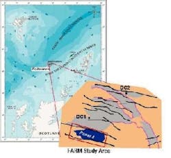
In 1995, BP and Shell, together with Schlum-berger, launched the 4D project known as Foinaven Active Reservoir Management (FARM). A key concern was whether the seismic would be repeatable enough to track the subtle changes in the reservoir. Consequently, the partners installed the first permanently emplaced deepwater seismic acquisition system over part of the Foinaven reservoir.
This allowed a comparison between different 4D technologies and their repeatability. The area covered is 7.5 sq km of Panel 4, a reservoir unit in the southern part of the Foinaven field.
FARM is probably the only example of a designer time-lapse survey in which the baseline survey was carried out before first oil. It is unique in having two baseline surveys prior to production using both towed streamer and permanent seabed array technology. In order to make both survey types as repeatable as possible, all the parameters that could be controlled in marine seismic acquisition were kept the same between the two vintages.
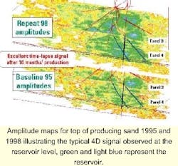
Baseline surveys of both seabed seismic and conventionally towed 3D seismic were acquired in 1995. In 1998, following 10 months of production, both towed and seabed surveys were repeated and all four data volumes were reprocessed. A clear time-lapse effect was observed on both the seabed and towed data, with a better 4D signal on the seabed data.
Reservoir changes
Changes were observed in the seismic response from the reservoir, which were interpreted as reservoir changes and which gave additional information about the reservoir.
Rock physics predicts that a drop in pressure will cause brightening. Since this brightening seems to occur over the whole reservoir, it is interpreted as good pressure communication in the whole compartment and little chance of bypassed oil.
The time-lapse images also suggest why a water injector was not performing well. The time-lapse seismic showed that the reservoir around the injector was unchanged, due either to excellent pressure support from the aquifer or poor connection to the producers. Injector performance supports the latter interpretation.
Other qualitative information about the reservoir was extracted from the amplitude maps. Where there are changes on one side of a fault and not the other, the fault is sealing. Effectiveness of dual completions can be examined without well intervention, and possible bypassed oil zones can be identified.
Measuring repeatability
After the first re-shoot, four different datasets were available over the target area. The seismic in the area is dominated by multiples and the key to processing success is a effective demultiple of the data. Processing of the datasets was optimized individually to produce four final migrated 3D volumes. Before using these volumes in time-lapse interpretation, any difference between the surveys of different vintages needed to be minimized.
The origins of these differences are all the uncontrollable factors in marine seismic, like waves, feathering, and water velocities. How-ever, most of the subsurface is unchanged between surveys of different vintages and this information can be used to analyze repeatability, as well as to take out some of the survey differences.
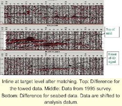
The 4D signal is clearly observable on the difference cubes because the 4D signal is larger than the largely coherent 4D noise. Different methods were used to estimate the repeatability between the two surveys post-stack and to measure the effect of different perturbations on the match between the surveys. We used:
- Predictability - a method used when matching borehole seismic data to surface seismic, independent of relative amplitudes and difference in wavelets.
- Interpretation of key horizons, comparing times and amplitudes
- RMS ratios and the effect of different perturbations on the relative RMS for the difference cubes normalized.
The numbers that we got from the different repeatability measures are not comparable as they respond to different attributes of the 4D signal and noise. However, as a relative measure of improvements from different perturbations, the different methods gave the same answer, although with different sensitivities.
Calibration
Cross-matching different 3D surveys is common, but is not really desirable unless there are some known global differences between the two surveys. Minimizing the residual in one window of the data does not necessarily provide an improvement at the target level. We were expecting to see a minimal need for cross-matching on both of the FARM data sets, as they are purposely designed for 4D seismic.
Several perturbations must be considered, starting with the survey-wide perturbations applied to all the data. Survey-wide perturbations include lateral shifts, bulk phase shifts, and global amplitude scaling. No survey-wide perturbation was deemed necessary. The trace-by-trace perturbation operators examined were time shifts, phase shifts, relative amplitude scaling, and matching filter. The final 4D processing approach included:
- The time and phase shifts were derived from the predictability analysis as shifts that maximize the predictability between the vintages.
- The same horizon(s) were interpreted on the two vintages of data and the difference was compared with the time shifts from the predictability analysis.
- As the predictability analysis is independent of relative amplitude between the two vintages, a scaling factor between the two vintages was obtained. The scaling factor(s) obtained this way are compared with the relative amplitude of an unchanged marker between the two surveys.
- Assessing the impact of the perturbation operator was done by computing normalized RMS in order to find the best combination of time shifts, phase shifts, and scaling strategy.
- Finally the difference cubes were examined and the possibility of improving the results through matching filters was evaluated.
Comparing the two vintages using matching filters was tested, but did not give clear, consistent improvements on the residual seismic. The final perturbations on the seabed data were only a bulk-time shift of 1.5 ms, while on the towed data it was trace-by-trace: time-shift, phase-shift, and scaling, based on relative RMS amplitudes.
Seabed versus towed
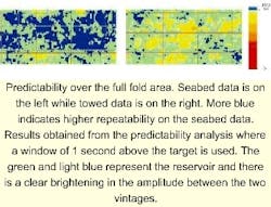
Less perturbation was needed to match the two vintages for the seabed data than for the towed data showing that the repeatability is better for seabed data. Another indicator is calculated from the predictability analysis. The predictability histogram for the seabed data has more data above 95% than the towed data. The average number for this full-fold area is 95% for seabed and 92% for towed data, which we interpret as the repeatability between the two vintages. Looking at the residual signal after matching, we get similar results for the comparison between the seabed and the towed data.
The final output of the 4D processing is the difference cubes, which can then be used both for quality control of horizon attributes extracted from each survey vintage and for direct interpretation of the time-lapse signal.
One disadvantage of placing hydrophones on the seabed is that the seabed multiple-to-primary ratio is much higher than for the towed data. To do a fair comparison between the two techniques, we need to consider the relative multiple problem as well as the acquisition effort. If we accept that the demultiple is the limiting factor for this 4D dataset, then the seabed data problem was roughly 10 times harder than for the towed data.
Conclusions
From the analysis, we see that a very good match can be obtained by a simple time-shift between the two seabed surveys, leaving the time-lapse signal as a clearly defined event in the sand under production. This time-lapse signal was interpreted as changes in the reservoir. The time-lapse signal also shows clearly on the towed data, where a trace-by-trace time, phase, and amplitude match was applied to obtain the best match. It should be noted that no survey-wide matching was deemed necessary.
Neither was a significant wavelet difference found between the two surveys. As expected, the seabed data had a higher repeatability than the towed data, even though the acquisition effort is less on the seabed survey and the water bottom multiple seen by the seabed hydrophone array is stronger than the multiples seen by the towed hydrophones.
A future permanent installation would likely benefit from easier, more effective demultiple processing, and possibly broader band P-wave images, using dual, or four-component sensors. Horizontal geophones would also allow access to the shear wavefield for greater control over elastic reflectivity, which would allow separation of pressure-related reservoir changes from fluid-related changes.
References
A complete list of references is available from the author.
Acknowledgement
The contributions of many in BP, Shell and Schlumberger have made the FARM program possible. BP and Shell provided permission to publish this article.
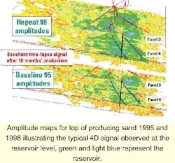
Amplitude maps for top of producing sand 1995 and 1998 illustrating the typical 4D signal observed at the reservoir level, green and light blue represent the reservoir.
