New noise level calculation unlocks 4D subsalt imaging

Shown here is the 3D noise map (A) and 4D noise map (B) for Field 1 in the deepwater GoM. The white dotted line indicates the field outline, while the black line indicates salt canopy edge, where the northern part is subsalt. The contours highlight steep dips and faults. (All images courtesy BP)

Instead of comparing one dataset to another in NRMS, to calculate 3DNRMS, a dataset is compared to a smoothed version of itself. This smoothed version is created by flattening the data along a horizon and applying a 3D average smoothing function. If the reflectors are parallel to the horizon and there is no noise in the data, the resulting 3DNRMS is zero. If there is additional noise in the data, the 3DNRMS goes up.

The 3DNRMS maps and SNR maps are very comparable.Unfortunately, real geological events with a high spatial frequency, such as faulting or stratigraphy, show up as 3D noise. On the other hand, coherent noise events can show up as low 3D noise. Examples are multiples or coherent subsalt events such as shear wave modes. These events are an issue with which all 3D noise levels measurements struggle, so the 3D noise map has to be carefully constructed and checked.

Of the 3D noise measures studied, 3DNRMS is preferred because it is independent of amplitude strength. Therefore, it not only provides a good 3D noise map within a field, but can also be used to compare different processing flows and different fields to each other. The other advantage is that when 3D and 4D noise are compared, the exact identical horizons and zones of interest can be used.

Noise comparison

Both 3D and 4D noise are affected by a large number of variables. All of the following parameters affect the amount of noise in the final dataset:

• Geology
• Reflection strength
• Illumination
• Processing
• Post-processing analysis
• Frequency content
• Overburden characteristics
• Acquisition style
• Fold
• Velocity model.

Note that all of these parameters affect both the 3D and 4D noise in a similar manner. For example, an incorrect velocity model results in both a lower quality 3D and a lower quality 4D image.

Of course, there are more factors impacting the 4D noise than the 3D noise. For example: source-receiver repeatability, source signature, water velocity or other statics, and consistent 4D processing.

The observations presented here are valid for any given acquisition and processing style, and qualitatively, the forward predictions are valid. However, to make quantitative forward predictions based on these comparisons, the time-lapse data of the fields must have similar acquisition and processing styles.

Correlations between 3D and 4D noise have historically been made by others. All show a clear relationship between SNR and NRMS.

This relationship was tested on data obtained from a field in thedeepwater GoM, then used in a forward prediction mode for 4D feasibility studies and future time-lapse acquisition.

Field observations

The deepwater GoM time-lapse data was acquired using deepwater nodes with excellent source-receiver repeatability characteristics. Then, the data set was processed using the most recent processing technology.

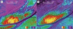
Shown here are 3D (labeled A) and 4D (labeled B) noise maps over Field 1, just above the main reservoir level. The northern part of this field is subsalt. Both maps are generated using the same horizon and the same interval. A strong correlation between the two maps can be observed. Both images show a strong impact of the structure, the illumination and the salt on the data quality. To the north, where the reservoir goes subsalt, the noise increases for both the 3D and 4D cases. The steep dips on the south flank of the reservoir are poorly imaged, resulting in high noise levels for both maps. These two maps of 3D and 4D noise have a high correlation with a coefficient of determination (R2) of 0.74.

Predictive mode

Next, the observations were used in a predictive mode to estimate noise levels in other subsalt fields that do not yet have 4D seismic data. In previous 4D feasibility workflows, one 4D noise level is used to estimate if the 4D signal is strong enough to get above the background noise level. This works well in extra salt areas and regions where enough calibration points of 4D noise levels from other time lapse surveys are available. However, it is much harder to estimate expected noise levels in the subsalt, especially since some areas have much worse data quality than others. Choosing one 4D noise level for both subsalt and extra salt seems to be too simplistic of an approach.

The following methodology is proposed for generating spatially varying 4D noise maps. A 3D noise level map is generated from the existing 3D dataset. The correlation between 3D and 4D noise levels is then used to make a prediction of the expected 4D noise level.

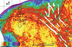
This workflow has been applied to Field 2. Here, predicted 4D noise levels are shown for both the extra salt and subsalt portions of this field, indicating where in the field issues are expected to allow a good 4D signal. The prediction is especially helpful in the area at the edge of salt, where it would not make sense to have a sharp jump in 4D data quality at this exact point. This new map shows a more gradual transition of 4D noise levels from extra salt to subsalt and not a discrete boundary.

Predicted NRMS levels for Field 2 are depicted in this image. The black line indicates the edge of the salt canopy, where the northern part is subsalt.

Degrading of the 4D noise levels is visible beyond the salt edge, which continues even further beneath the salt body.

This first step is a qualitative method that describes which parts of field are the most likely to have good 4D data quality. The next step is to predict the 4D noise level in a quantitative method by establishing a ratio between 3D and 4D noise from other fields with similar acquisition and processing, and then using this ratio to convert the 3D noise map into a predicted 4D noise map.

For the quantitative workflow, a good range of datasets with equal acquisition and processing characteristics is needed, which might not be available. A simpler method to get a more quantitative comparison is to calibrate the predicted 4D noise map in an extra salt area to the expected 4D noise ratios from regional experience. For example, in the figure above, the extra salt NRMS value could be calibrated to a value around 6%. This value is the expected NRMS value in 4D data in an extra salt area acquired with nodes.

Conclusion

Both 3D and 4D noise were defined, and 3DNRMS was introduced as a new tool to show 3D noise levels. For fields in the deepwater GoM, a good correlation between 3D and 4D noise levels was shown.

The correlation between 3D and 4D noise levels can be used to predict where low 4D noise levels can be expected in other subsalt fields, where the 3D seismic data quality within a field varies strongly due to the subsalt imaging issues.

An important conclusion that can be drawn from the correlation between 3D and 4D noise is that 4D noise levels could be reduced similarly to 3D noise level reduction. By acquiring more offsets and azimuths; improving the velocity model; and improving the imaging and all other methods that result in better 3D images, 4D noise levels would also be reduced. This is easier said than done, since 3D imaging is already pushed as much as possible. In addition, these methods must be applied in a 4D-consistent manner, which might be difficult for some of the complicated acquisition styles.

As more datasets are tested with the observations that were made in this paper, the 4D subsalt problem will hopefully be solved.

The author

Jean-Paul van Gestel is the lead seismic analyst of BP’s Gulf of Mexico Production Team in Houston, focusing on time-lapse analysis and attribute analysis, specifically for subsalt fields. He has worked for BP for 15 years, in Upstream Technology, Brazil Exploration, and on the Life of Field Seismic (LoFS) Project for BP Norway. A member of the Society of Exploration Geophysicists and the European Association of Geoscientists and Engineers, Van Gestel was the first author of a publication on the integration of LoFS data that won SEG’s “The Leading Edge” best paper award in 2008. He also served on the EAGE distinguished lecture program in 2010. He and his colleagues won the Bonarelli award for best oral presentation at the 2009 EAGE meeting. van Gestel received his M. Sc. degree in Geophysics from the Delft University of Technology in 1996 and his Ph. D. in Geophysics from The University of Texas at Austin in 2000.

Acknowledgments

The author wishes to thank BP colleagues for discussion and feedback, as well as BP, BHP Billiton, and ExxonMobil for permission to show the data. Based on a paper presented at the SEG annual meeting held in New Orleans, Oct. 18-23, 2015.